GNSS-Aided Visual-Inertial Odometry: Accurate Frame Initialization for Improved Localization
Accurate localization is crucial for mobile autonomous systems. While Visual-Inertial Odometry provides a robust navigation solution, it can suffer from drift over time and large distances. GNSS-aided VIO offers a solution to the problem of drift but requires an initial estimate of the local reference frame, which is often challenging to establish accurately and consistently. Current methods can result in large discrepancies in global to local frame initialization errors due to sub-optimal thresholds such as time or distance traveled. This work addresses this issue by developing a novel method for determining when to initialize the global to local transformation using user-specified desired error values and further refining the transformation heading using online estimates. This proposed approach is flexible in the number of sensors used, ensures consistent localization accuracy across various scenarios, and outperforms existing solutions, all as verified through Monte Carlo simulations and experimental data. An example of the algorithm presented as well as the simulation code is available online at https://github.com/unmannedlab/ekf_cal.
Introduction and Related Work
For any mobile autonomous system, accurate localization is paramount to operation. The use of IMU and cameras in a VIO system can provide robust navigation in a wide variety of environments by combining proprioceptive and exteroceptive sensing in a low-cost yet relatively high-quality manner. However, on their own, VIO systems cannot prevent long-term drift and global positioning error due to the well understood four unobservable degrees of freedom that define the origin and heading of the local VIO reference frame [1].
A common solution to this is the use of SLAM, which makes use of loop-closure constraints to eliminate long term drift and origin placement errors [2,3]. These algorithms, in general, are very promising in their high translational and rotational accuracies in a wide variety of environments using various sensor combinations. This, however, comes at the costs of additional memory and computational throughput requirements, which precludes the use of these algorithms on many devices. Additionally, the ability to perform loop closure is limited in single directional or non-overlapping trajectories, which would therefore still be subject to drift.
Alternatively, the additional degrees of freedom can be made observable using a GNSS receiver in a Kalman filter-based framework [4-6]. The measurements from GNSS provide global, drift-free position estimates using computationally lightweight and inexpensive sensors with the primary drawback being the limitations on where the measurements can be used or trusted. For example, there are many environments such as indoors, underground, or underwater where GNSS measurements are unavailable. Additionally, there are environments such as in urban canyons where GNSS measurements are available but cannot be trusted due to high multipath errors. Therefore, it is necessary to consider the intermittent availability of GNSS measurements. Minimally, IMU and GNSS measurements can be used to estimate ego motion, but many incorporate camera measurements as well to add robustness to the previously mentioned issues [7,8]. and GNSS produces antenna position measurements in a global frame. Typically this is latitude, longitude, and altitude within the WGS-84 reference frame. While these can be freely transformed into any other global frame ${G}$, in order to transform these measurements into a local flat reference frame ${L}$ and then to a body-fixed frame ${B}$, a local reference point must be provided. This is necessary to incorporate these measurements into the VIO system. Additionally, if the local VIO frame ${L}$ is not aligned with the global frame ${G}$ (beyond the alignment of the gravity vector in the up direction), an additional heading rotation must be known. This is the source of the previously mentioned four degrees of freedom of a VIO localization system. It is desirable to first accurately initialize the frame transformation between the global frame and the local VIO frame to prevent unnecessary drift in the VIO output as initial estimation errors are eliminated.
A common solution is to set the first GNSS measurement as the local frame origin and utilize a bearing measurement, such as differential GNSS, to set the local frame heading. When available, this is a fairly robust solution, given an adequate a priori estimate of the GNSS antennae positions. The primary drawback with this method is inconsistent initialization due to errors in the first position and bearing measurement. Some, such as [9,10], have utilized magnetometers for the bearing measurement. In addition to being inconsistent, such as system is subject to hard and soft iron effects which are difficult to remedy without an in-place magnetometer calibration.
A more robust solution therefore is to utilize the GNSS measurements to initialize the local frame. SLAM frameworks can calculate a sliding window estimate of the local frame origin and rotation parameters using non-linear estimation [11,12]. Some filter-based methods use a LSS method to calculate a constant local frame initialization once the trajectory length has exceeded a user-specified distance [13]. However, this may produce inconsistent initialization errors and system drift due to heading alignment errors. Building upon this method, [6] showed the global frame to local frame heading rotation is observable in many trajectories, and can therefore be calibrated online. This improved localization accuracy for longer trajectories, but still is subject to inconsistent initialization errors which this work seeks to remedy.
In terms of simulation software, the current state-of-the-art open-sourced online estimation filter and simulator is OpenVINS [14]. It provides an implementation of the filter developed in [13] alongside a one-at-a-time runner that simulates a single IMU and multiple cameras by generating accelerations from splines and features from globally tracked, static points. One limitation of this method of simulation is it cannot confirm overall convergence and stability of a filter, but rather just the success of a single run. This works seeks to expand on this methodology using Monte Carlo testing for filter convergence.
In this work, I propose a novel global frame initialization thresholds for a tightly-coupled, online calibrating GNSS-VIO that is multi-IMU, multi-camera, and multi-GNSS. Our specific contributions are
- I propose probabilistic global to local frame initialization thresholds that are more consistent in resultant initialization errors and function independently of measurement noise and rates.
- I propose similar thresholding to estimate when an online calibration update of the global to local frame heading should be performed compared to a reduced state update of just the position.
- I have open-sourced an implementation of this filter and thresholding technique in addition to a Monte Carlo simulation architecture for this online calibrating GNSS-VIO, available online at https://github.com/unmannedlab/ekf_cal.
Algorithm Description
State Definition
The system is defined as a rigidly attached combination of at least one IMU, camera, and GNSS receiver, where the addition of redundant sensors can improve localization accuracy and add robustness to sensor drop outs and failures. Therefore, the composite state combines the states of the body with each of the extrinsic and intrinsic calibration parameters for the three sensors supported by the filter. The state is defined as
\[\boldsymbol{x} = \begin{bmatrix} \boldsymbol{x}_{B} & \boldsymbol{x}_{I} & \boldsymbol{x}_{G} & \boldsymbol{x}_{C} \end{bmatrix}\]where \(\boldsymbol{x}_{B}\) is the body state, \(\boldsymbol{x}_{I}\) is the IMU composite state, \(\boldsymbol{x}_{G}\) is the GNSS composite state, and \(\boldsymbol{x}_{C}\) is the camera composite state. The body state $\boldsymbol{x}_{B}$ is defined as,
\[\boldsymbol{x}_{B} = \begin{bmatrix} {}^{L}\boldsymbol{p}_{B} & {}^{L}\boldsymbol{p}_{B} & {}^{L}\boldsymbol{a}_{B} & {}^{L}_{B}{q} & {}^{L}\boldsymbol{\omega}_{B} & {}^{L}\boldsymbol{\alpha}_{B} \end{bmatrix}\]where \({}^{L}\boldsymbol{p}_{B}\) is the body position, \({}^{L}\boldsymbol{p}_{B}\) is the body velocity, \({}^{L}\boldsymbol{a}_{B}\) is the body acceleration, \({}^{L}_{B}{q}\) is the body orientation, \({}^{L}\boldsymbol{\omega}_{B}\) is the body angular velocity, \({}^{L}\boldsymbol{\alpha}_{B}\) is the body angular acceleration, \(\{B\}\) represents the moving body-fixed frame, and \(\{L\}\) represents the static local frame. The IMU state $\boldsymbol{x}_{I}$ is defined as,
\[\boldsymbol{x}_{I} = \begin{bmatrix} \begin{bmatrix} {}^{B}\boldsymbol{p}_{I} \\ {}^{B}_{I}{q} \\ \boldsymbol{b}_a \\ \boldsymbol{b}_\omega \end{bmatrix}_0^T & ... & \begin{bmatrix} {}^{B}\boldsymbol{p}_{I} \\ {}^{B}_{I}{q} \\ \boldsymbol{b}_a \\ \boldsymbol{b}_\omega \end{bmatrix}_{N_i}^T \end{bmatrix}\]where \({}^{B}\boldsymbol{p}_{I}\) is the IMU position, \({}^{B}_{I}{q}\) is the IMU orientation, \(\boldsymbol{b}_a\) is the IMU accelerometer bias, \(\boldsymbol{b}_\omega\) is the IMU gyroscope bias, and \(N_i\) is the number of IMU. The GNSS state \(\boldsymbol{x}_{G}\) is defined as,
\[\boldsymbol{x}_{G} = \begin{bmatrix} {}^{G}{L}{\theta} & {}^{B}\boldsymbol{p}_{A_{0}} & ... & {}^{B}\boldsymbol{p}_{A_{N_g}} \end{bmatrix}\]where \({}^{G}{L}{\theta}\) is the heading rotation from the local to the global frame, \({}^{B}\boldsymbol{p}_{A}\) is the GNSS antenna position, and \(N_g\) is the number of GNSS antenna. Lastly, the camera state \(\boldsymbol{x}_{C}\) is defined as,
\[\boldsymbol{x}_{C} = \begin{bmatrix} \begin{bmatrix} {}^{B}\boldsymbol{p}_{C} \\ {}^{B}_{C}{q} \\ \boldsymbol{x}_{A_{t-1}} \\ \vdots\\ \boldsymbol{x}_{A_{t-N_A}} \end{bmatrix}_0^T & ... & \begin{bmatrix} {}^{B}\boldsymbol{p}_{C} \\ {}^{B}_{C}{q} \\ \boldsymbol{x}_{A_{t-1}} \\ \vdots\\ \boldsymbol{x}_{A_{t-N_A}} \end{bmatrix}_{N_c}^T \end{bmatrix}\]where \({}^{B}\boldsymbol{p}_{C}\) is the camera position, \({}^{B}_{C}{q}\) is the camera orientation, \(N_c\) is the number of GNSS antenna, and the $N_A$ augmented state clones are defined as
\[\boldsymbol{x}_{A} = \begin{bmatrix} {}^{L}\boldsymbol{p}_{B} & {}^{L}_{B}{q} & {}^{B}\boldsymbol{p}_{C} & {}^{B}_{C}{q} \end{bmatrix}\]where for each augmented state, \({}^{L}\boldsymbol{p}_{B}\) is the body position, \({}^{L}_{B}{q}\) is the body orientation, \({}^{B}\boldsymbol{p}_{C}\) is the camera position, and \({}^{B}_{C}{q}\) is the camera orientation.
State Prediction
As shown in [15], when performing online filtering of multiple IMU, the prediction step of the Kalman filter is derived from the following continuous-time dynamic system of equations
\[\begin{array}{lcl} {}^{L}\dot{\boldsymbol{p}}_{B} = {}^{L}\boldsymbol{p}_{B} & ~ & {}^{L}_{B}\dot{q} = \frac{1}{2} \Omega(\boldsymbol{}^{L}\boldsymbol{\omega}_{B}) {}^{L}_{B}{q} \\[0.5ex] {}^{L}\dot{\boldsymbol{v}}_{B} = {}^{L}\boldsymbol{a}_{B} - \mathcal{C}\left({}^{L}_{B}{q}\right) \boldsymbol{g} & ~ & {}^{L}\dot{\boldsymbol{\omega}}_{B} = {}^{L}\boldsymbol{\alpha}_{B} \\[0.5ex] {}^{L}\dot{\boldsymbol{a}}_{B} = \boldsymbol{0} & ~ & {}^{L}\dot{\boldsymbol{\alpha}}_{B} = \boldsymbol{0} \end{array}\]where \(\mathcal{C}(q)\) is the rotation matrix of quaternion \(q\), the function \(\Omega\) is defined as
\[\Omega(\boldsymbol{\omega}) = \begin{bmatrix} - \left\lfloor{\boldsymbol{\omega}}\right\rfloor_{\times} & \boldsymbol{\omega} \\ \boldsymbol{\omega}^T & 0 \end{bmatrix}\]and the cross product matrix function \(\left\lfloor \right\rfloor_{\times}\) is defined as
\[\left\lfloor {\boldsymbol{\omega}} \right\rfloor_{\times} = \begin{bmatrix} 0 & -\omega_z & \omega_y \\ \omega_z & 0 & -\omega_x \\ -\omega_y & \omega_x & 0 \end{bmatrix}\]As such, the discrete-time state transition function is defined as
\[\boldsymbol{f} \left( \boldsymbol{x} \right) = \left[ \begin{array}{ccl} {}^{L}\boldsymbol{p}_{B} & + & {}^{L}\boldsymbol{p}_{B} \Delta t \\ {}^{L}\boldsymbol{p}_{B} & + & ({}^{L}\boldsymbol{a}_{B} - \mathcal{C}\left({}^{L}_{B}{q}\right) \boldsymbol{g} ) \Delta t \\ {}^{L}\boldsymbol{a}_{B} & & \\ {}^{L}_{B}{q} & \otimes & q(\hat{\boldsymbol{\omega}}_{k-1} \Delta t) \\ {}^{L}\boldsymbol{\omega}_{B} & + & \hat{\boldsymbol{\alpha}} \Delta t \\ {}^{L}\boldsymbol{\alpha}_{B} & & \\ \boldsymbol{x}_{I} & & \\ \boldsymbol{x}_{G} & & \\ \boldsymbol{x}_{C} & & \end{array} \right]\]where \(\boldsymbol{g}\) is the gravity vector and \(\otimes\) is quaternion multiplication. The linearized state transition matrix, $\boldsymbol{F}$, is defined as
\[\boldsymbol{F} = \frac{\partial f}{\partial \boldsymbol{x}}\]and is fully derived in [15]. The state transition function and state transition matrix are then used to predict the state and covariance, respectively
\[\hat{\boldsymbol{x}}_{k|k-1} = \boldsymbol{f}(\hat{\boldsymbol{x}}_{k-1|k-1})\] \[\boldsymbol{P}_{k|k-1} = \boldsymbol{F}_k \boldsymbol{P}_{k-1|k-1} \boldsymbol{F}_k^T + \boldsymbol{Q}_k\]where the process noise $\boldsymbol{Q}$ is calculated offline and is a constant.
Measurement Model
The GNSS antenna are assumed to be rigidly attached to the body with an uncertain extrinsic position offset in the body frame between to the origin of the antenna. As the post-initialized GNSS makes measurements in the global frame ${G}$, the model for each GNSS measurement is
\[\mathbf{z} = \begin{bmatrix} {}^{G}\boldsymbol{p}_{A} \end{bmatrix}\] \[\hat{\mathbf{z}} = \begin{bmatrix} \mathcal{C}\left({}^{G}_{L}\hat{\theta}\right) \left( {}^{L}\hat{\boldsymbol{p}}_{B} + {}^{L}_{B}\hat{q} {}^{B}\hat{\boldsymbol{p}}_{A} \right) \end{bmatrix}\]where \({}^{G}\boldsymbol{p}_{A}\) is the true antenna position, \({}^{G}_{L}\hat{\theta}\) is the heading rotation from the local frame to the global frame, \({}^{L}\hat{\boldsymbol{p}}_{B}\) is the body position, \({}^{L}_{B}\hat{q}\) is the body orientation, and \({}^{B}\hat{\boldsymbol{p}}_{A}\) is the position of the GNSS antenna. With this definition of the measurement model, it is possible to develop a method of local frame initialization and the measurement update equations.
Local Frame Initialization
Before GNSS measurements can be utilized in an online calibration estimator, there must first exist a transformation between global and local coordinates. This comes in the form of defining the origin of an local frame in global coordinates, and estimating an initial global to local heading angle. To perform the global to local frame initialization, it is necessary to have an a priori estimate of the location of the GNSS antenna in the body frame ${}^{B}\hat{\boldsymbol{p}}_{A}$ that can be utilized in the initialization process outlined in the following algorithm.
| Algorithm: Global to Local Frame Initialization |
|---|
| 1: procedure \(\text{AttemptInitialization} \left({}^{G}\boldsymbol{P}_{A}, {}^{L}\hat{\boldsymbol{P}}_{B} \right)\) |
| 2: \(~~~~ {}^{G}\hat{\boldsymbol{p}}_{L}, {}^{G}_{L}\hat{\theta} \gets \text{KabschUmeyama}({}^{G}\boldsymbol{P}_{A},~ {}^{L}\hat{\boldsymbol{P}}_{B})\) |
| 3: \(~~~~ \tilde{\boldsymbol{p}} \gets \text{PositionResiduals}({}^{G}\boldsymbol{P}_{A},~ {}^{L}\hat{\boldsymbol{P}}_{B},~ {}^{G}\hat{\boldsymbol{p}}_{L},~ {}^{G}_{L}\hat{\theta})\) |
| 4: \(~~~~ \tilde{\theta} \gets \text{HeadingResiduals}( {}^{G}\boldsymbol{P}_{A},~ {}^{L}\hat{\boldsymbol{P}}_{B},~ {}^{G}\hat{\boldsymbol{p}}_{L},~ {}^{G}_{L}\hat{\theta})\) |
| 5: \(~~~~ \sigma_{p} \gets \text{MeanStandardDeviation}(\tilde{\boldsymbol{p}})\) |
| 6: \(~~~~ \sigma_{\theta} \gets \text{MeanStandardDeviation}(\tilde{\theta})\) |
| 7: return \({}^{G}\hat{\boldsymbol{p}}_{L},~ {}^{G}_{L}\hat{\theta},~ \sigma_{p},~ \sigma_{\theta}\) |
| 8: end procedure |
With the a priori estimate of the GNSS antenna position(s), measurements and body position in the local frame ${}^{L}\hat{\boldsymbol{p}}_{B}$ are saved to attempt the initialization procedure with each additional measurement. Because the gravity vector is aligned between the global and local frames, there are only 4 degrees of freedom of this estimate. With this assumption, I developed the following procedure for initializing both the fixed local origin in the global frame and the initial estimate of the global to local heading rotation.
where \({}^{G}\boldsymbol{P}_{A}\) is the matrix of measured antenna positions in the global ${G}$ frame, \({}^{L}\hat{\boldsymbol{P}}_{B}\) is the matrix of estimated body positions in the local frame, \({}^{G}\hat{\boldsymbol{p}}_{L}\) is the estimated origin of the local frame in the global frame, \({}^{G}_{L}\hat{\theta}\) is the estimated heading of the local frame to the global frame, \(\boldsymbol{r}_p\) is a vector of the position residuals, \(\boldsymbol{r}_\theta\) is a vector of the angle residuals, \(\epsilon_{p}\) is the standard deviation of the estimated position of the local frame, \(\epsilon_{\theta}\) is the standard deviation of the estimated heading of the local frame, \(\epsilon_{p_{th}}\) is the position error threshold, \(\epsilon_{\theta_{th}}\) is the angular error threshold, and \(\{G\}\) is the global frame.
Thresholding
To initialize the local frame, a three-dimensional translation and one-dimensional rotation are calculated using the well known Kabsch-Umeyama algorithm [16,17] using singular value decomposition as was done in [18]. These estimates minimize the root mean squared deviation between the body position estimates and the GNSS position measurements. However, this method does not produce any information on the transformation’s expected error. Therefore, I propose a method of thresholding using the estimated transformations. With these estimates, the reprojection errors are calculated for both the translational and rotational space. The reprojection errors are separated due to the possibility of having low translational uncertainty but high rotational uncertainty. This can occur in the case of initially stationary data, which can result in drift if the motion ever becomes non-stationary.
In order to introduce more consistent initialization, I propose the use of thresholds with respect to the standard deviation of the estimate. To calculate these standard deviations, the measurement residuals are first calculated as
\[\begin{align} \tilde{\boldsymbol{p}} & = {}^{L}\hat{\boldsymbol{p}}_{B} -\mathcal{C}\left({}^{G}_{L}\hat{\theta}\right)^T \left({}^{G}\boldsymbol{p}_{A} - {}^{G}\hat{\boldsymbol{p}}_{L}\right) \\[0.5ex] \tilde{\theta} & = \tan\left(\frac{|{}^{L}\hat{\boldsymbol{p}}_{B} \times \tilde{\boldsymbol{p}}|}{|{}^{L}\hat{\boldsymbol{p}}_{B}|}\right) \end{align}\]The sets of residuals across many measurements can be used to calculate the expected standard deviation in the position and heading distributions as follows.
\[\begin{align} \sigma_p & = \frac{1}{N} \sqrt{\sum_{i=1}^{N} |\tilde{\boldsymbol{p}}_i|^2} \\[0.5ex] \sigma_\theta & = \frac{1}{N} \sqrt{\sum_{i=1}^{N} \tilde{\theta}_i^2} \end{align}\]Once both the standard deviations are below the given thresholds, $\epsilon_{p_{th}}$ and $\epsilon_{\theta_{th}}$, the output of the Kabsch-Umeyama algorithm is used to marginalize the origin of the global frame and to initialize the dynamically estimated heading of the local frame.
An estimate of the number of measurements required to reach this threshold can be derived such that the expected number of GNSS measurements needed to initialize the origin of the global frame is
\[N_p = \frac{\sigma^2_{G}}{\sigma^2_{th}}\]where $N_p$ is the expected number of GNSS measurements, $\sigma_{G}$ is the standard deviation of the GNSS measurements, and $\sigma_{th}$ is the desired error threshold to initialize the global origin.
Unfortunately, a similar estimate cannot be derived for the angular threshold due to the dependency on the baseline distance. As such, initialization measurement counts can vary depending on the type of trajectory, where, intuitively, longer baseline distances lead to greater reductions in angular uncertainty and some trajectories lead to no reduction in angular uncertainty. This follows from [6] which discussed some types of degenerate motion that can prevent the initialization of the local frame heading, such as uniform circular motion.
Measurement Updates
To perform the typical extended Kalman update, the jacobian of the measurement with respect to the entire state is derived. The measurement Jacobian with respect to the body state is
\[\boldsymbol{H}_B = \begin{bmatrix} \boldsymbol{J}^{L}\boldsymbol{p}_{B} & \mathbf{0}_{3 \times 6} & \boldsymbol{J}^{L}_{B}{q} & \mathbf{0}_{3 \times 6} \end{bmatrix}\]where
\[\begin{split} &\boldsymbol{J}_{ {}^{L}\boldsymbol{p}_{B} } = \mathcal{C}\left({}^{G}_{L}\hat{q}\right) \\ &\boldsymbol{J}_{ {}^{L}_{B}{q} } = -\mathcal{C}\left({}^{G}_{L}\hat{q}\right) \mathcal{C}\left({}^{L}_{B}\hat{q}\right) \left\lfloor{}^{B}\hat{\boldsymbol{p}}_{A}\right\rfloor_{\times} \end{split}\]The measurement Jacobian with respect to the GNSS state is
\[\boldsymbol{H}_G = \begin{bmatrix} \boldsymbol{J}_{}^{G}{L}{\theta} & ... & {}^{i}{\boldsymbol{J}_{}^{B}\boldsymbol{p}_{A}} & ... \end{bmatrix}\]where
\[\begin{split} &\boldsymbol{J}_{}^{G}{L}{\theta} = -\mathcal{C}\left({}^{G}_{L}\hat{q}\right) \left\lfloor{}^{L}\hat{\boldsymbol{p}}_{B} + {}^{L}_{B}\hat{q} {}^{B}\hat{\boldsymbol{p}}_{A}\right\rfloor_{\times} \\ &{}^{i}{\boldsymbol{J}_{}^{B}\boldsymbol{p}_{A}} = \mathcal{C}\left({}^{G}_{L}\hat{q}\right) \mathcal{C}\left({ {}^{L}_{B}\hat{q}}\right) \end{split}\]and the GNSS antenna position jacobian \({}^{i}{\boldsymbol{J}_{}^{B}\boldsymbol{p}_{A}}\) aligns with the associated state of the measuring GNSS sensor \(i\). The remaining Jacobians with respect to the IMU and camera states (\(\boldsymbol{H}_{I}\) and \(\boldsymbol{H}_{C}\) respectively) are zero.
\(\boldsymbol{H}_{I} = \mathbf{0}_{3 \times 12N_I}\) \(\boldsymbol{H}_{C} = \mathbf{0}_{3 \times 6N_C}\)
Combining these four sub-state Jacobians produces the complete observation matrix.
\[\boldsymbol{H} = \begin{bmatrix} \boldsymbol{H}_{B} & \boldsymbol{H}_{I} & \boldsymbol{H}_{G} & \boldsymbol{H}_{C} \end{bmatrix}\]However, there may be very low observability of the global to local heading rotation. This arises when the GNSS position error exceeds the baseline distance traveled in the global frame. For example, if the GNSS horizontal standard deviation is 10 meters, but the system has only moved 5 meters, the heading has low observability and should not be updated. For measurements failing this condition, the observation matrix is reduced by assuming the heading rotation is fixed, and the online calibration is not performed. Therefore when the baseline distance traveled by the system is less than the GNSS measurement standard deviation, the Jacobian with respect to the local heading reference is set to zero.
\[|{}^{L}\boldsymbol{p}_{B}| < \sigma_{GNSS} \implies \boldsymbol{J}_{}^{G}{L}{\theta} = \mathbf{0}_{3 \times 3}\]With the observation matrix calculated, it is possible to calculate the measurement residual $\boldsymbol{y}$ and residual covariance $\boldsymbol{S}$
\[\boldsymbol{y}_k = \boldsymbol{z}_k - \hat{\boldsymbol{z}}_k\] \[\boldsymbol{S}_k = \boldsymbol{H}_k \boldsymbol{P}_{k|k-1} \boldsymbol{H}_k^T + \boldsymbol{R}_k\]The Mahalanobis distance test is used to reject outliers that exceed a given chi-squared threshold , $\chi^2$, as is typically done in EKF implementations.
\[\boldsymbol{y}_k^T \boldsymbol{S}_k^{-1} \boldsymbol{y}_k < \chi^2\]For measurements where this inequality is true, the typical Kalman update is performed
\[\boldsymbol{K}_k = \boldsymbol{P}_{k|k-1} \boldsymbol{H}_k^T \boldsymbol{S}_k^{-1}\] \[\hat{\boldsymbol{x}}_{k|k} = \hat{\boldsymbol{x}}_{k|k-1} \oplus \boldsymbol{K}_k \boldsymbol{y}_k\] \[\boldsymbol{P}_{k|k} = (\boldsymbol{I} - \boldsymbol{K}\boldsymbol{H}) \boldsymbol{P}_{k|k-1} (\boldsymbol{I} - \boldsymbol{K}\boldsymbol{H})^T + \boldsymbol{K}_k \boldsymbol{R}_k \boldsymbol{K}_k^T\]where the state composition $\oplus$ is defined as addition for vectors and quaternion multiplication for quaternions. Additionally, the covariance update is computed using the Joseph form for it’s balance of improved numerical stability and computational complexity [19]. The remaining measurement update equations for the IMU and camera measurements are derived in [15,20].
Simulated Results
In order to evaluate the proposed filter, an open sourced monte carlo simulation environment was utilized (available at https://github.com/unmannedlab/ekf_cal). Measurement streams were generated using the outline measurement model with additional Gaussian white noise in the sensor frame applied to the baseline truth model. Splines were used to generate continuously differentiable trajectories in both translational and rotational spaces.
First, the simulation was used to verify the efficacy of the local frame initialization error thresholding. This was done by sweeping the translational and rotational error thresholds input into the filter and computing the mean error across runs. The experiment was conducted using a 1000 run Monte Carlo set where variance was injected into parameters using the previously outlined error parameters and distributions. The approximately linear and unbiased plots for the translational and rotational errors show that the thresholding method correctly predicts the expected variance of the initialized local frame independent of measurement variance or update rate.
| Parameter | Std. Dev. | Units |
|---|---|---|
| ${}^{G}\boldsymbol{p}_{L}$ | 10 | m |
| ${}^{G}{L}{\theta}$ | 1 | rad |
| $a$ | 0.01 | m/s/s |
| $\omega$ | 0.001 | rad/s |
| $b_{a}$ | 0.01 | m/s/s |
| $b_{\omega}$ | 0.01 | rad/s |
| ${}^{B}\boldsymbol{p}_{A}$ | 0.1 | m |
| $f_{IMU}$ | 400 | hz |


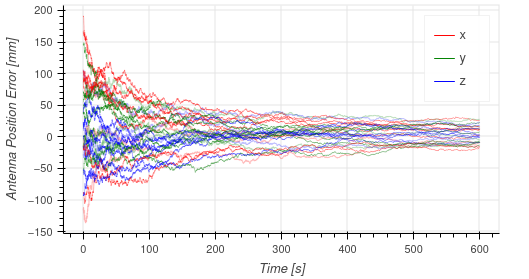
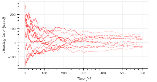
Additionally, the simulation Monte Carlo framework was used to verify the stability and accuracy of the proposed filtering methods. To do this, randomly sampled errors were injected to all initial state estimates for each run in a Monte Carlo set, which were then compiled to compute filter statistics. Results of the online estimation of both the GNSS antenna offset in the body frame as well as heading of the local frame are shown in the following two figures. These plots confirm the overall stability of the filter in addition to show the ability of the proposed filter design to reduce the antenna position error and local heading errors from 100 millimeters and 200 milliradians to 50 millimeters and 100 milliradians of error over the course of a ten minute simulation.
Experimental Results
In addition to Monte Carlo simulations, a physical experiment was performed using a VectorNav VN-300 IMU and dual-antenna GNSS, a VectorNav VN-100 IMU, and two Basler Ace cameras mounted on a ground vehicle using the mounting pattern shown in the figure below. Calibration parameter priors for the online filter were calculated using hand measurements. Ground truth for the GNSS antenna and local frame heading rotation were calculated prior to the experiment using the VN-300’s onboard antenna calibration and GNSS compass over the course of a 20 minute trajectory. The thresholds to initialize the local frame global position and heading were 100 millimeters and 100 milliradians.

The resulting experiment over the trajectory shown in the following figure compares the resulting trajectories of four different global to local frame transformation initialization methods with the resulting mean position error of each method outlined in the following table. The first point method represents using the first measured magnetometer heading to initialize the local frame. The distance-based method refers to the use of a 100 meter baseline distance threshold to perform a LSS estimate of the transformation, which is the current state of the art thresholding method. The proposed-fixed refers to using the initial value given by the method proposed in this paper without online estimation, and the proposed-online shows the additional reduction in error through the use of online estimation of the global to local heading.
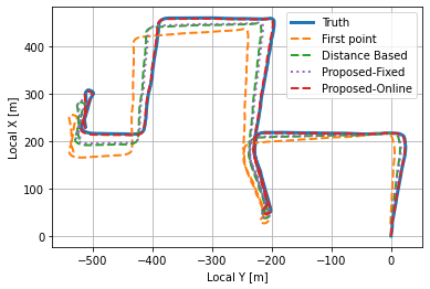
| Method | Mean Position Error [m] |
|---|---|
| Distance Based | 18.8 |
| Proposed-Fixed | 16.1 |
| Proposed-Online | 1.9 |
Additionally, the online estimator had had antenna position and local frame heading errors shown in the following two figures.
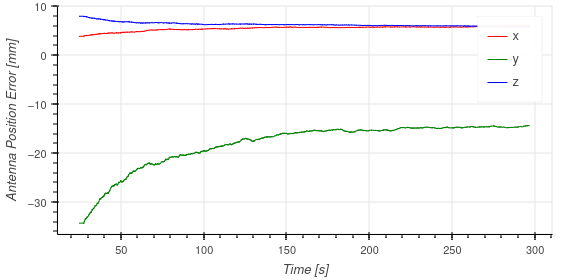
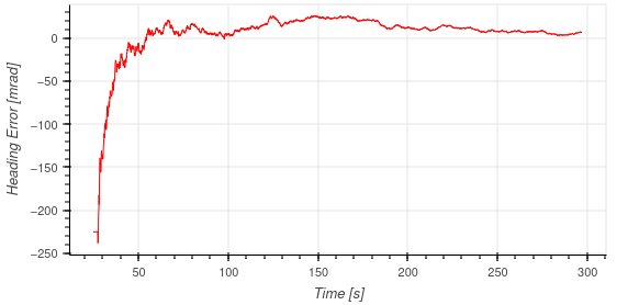
The reduction of error over the course of the experiment is consistent with the simulation results and verifies the stability and accuracy of the filter framework. However, the initial local frame rotation error was 225 milliradians, which is greater than the desired 100 milliradian angular threshold set. However, due to the probabilistic nature of the thresholds provided, this is not an unexpected result. Additionally, as outlined in the results table, the additional inclusion of the online local heading calibration on top of the thresholding method provides better localization accuracy due to the reduction of error in both the antenna position and local frame heading over the course of the experiment.
Conclusions
In this work, I have presented consistent methods for initializing an online calibrating GNSS-VIO filter. Whereas existing metrics to initialize the global to local frame rotation for GNSS measurements are heuristic, I present probabilistic methods based on the expected mean error. Through the use of Monte Carlo simulations, I have shown that the proposed methods for thresholding the GNSS initialization are accurate in their error estimations as is the method for estimating the number of measurements required to initialize below a given position error. Experimental data corroborates these findings, while also confirming the stability and accuracy of the filter. Finally, the code used to run the presented Monte Carlo simulations and experiments is open-source and available online at https://github.com/unmannedlab/ekf_cal.
References
- J. Kelly and G. S. Sukhatme, “Visual-inertial sensor fusion: Localization, mapping and sensor-to-sensor self-calibration,” The International Journal of Robotics Research, vol. 30, no. 1, pp. 56–79, 2011. [Online]. Available: https://doi.org/10.1177/0278364910382802
- T. Qin and S. Shen, “Online temporal calibration for monocular visual- inertial systems,” in 2018 IEEE/RSJ International Conference on Intel- ligent Robots and Systems (IROS), 2018, pp. 3662–3669.
- C. Campos, R. Elvira, J. J. G. Rodrı́guez, J. M. M. Montiel, and J. D. Tardós, “Orb-slam3: An accurate open-source library for visual, visual–inertial, and multimap slam,” IEEE Transactions on Robotics, vol. 37, no. 6, pp. 1874–1890, 2021.
- Y. Lee, J. Yoon, H. Yang, C. Kim, and D. Lee, “Camera-gps-imu sensor fusion for autonomous flying,” in 2016 Eighth International Conference on Ubiquitous and Future Networks (ICUFN), 2016, pp. 85–88.
- W. Lee, K. Eckenhoff, P. Geneva, and G. Huang, “Intermittent gps-aided VIO: Online initialization and calibration,” in 2020 IEEE International Conference on Robotics and Automation (ICRA), 2020, pp. 5724–5731.
- J. Song, P. J. Sanchez-Cuevas, A. Richard, R. T. Rajan, and M. Olivares- Mendez, “Gps-vio fusion with online rotational calibration,” 2024.
- C. V. Angelino, V. R. Baraniello, and L. Cicala, “Uav position and atti- tude estimation using imu, gnss and camera,” in 2012 15th International Conference on Information Fusion, 2012, pp. 735–742.
- T. Oskiper, S. Samarasekera, and R. Kumar, “Multi-sensor navigation algorithm using monocular camera, imu and gps for large scale aug- mented reality,” in 2012 IEEE International Symposium on Mixed and Augmented Reality (ISMAR), 2012, pp. 71–80.
- J. Almazán, L. M. Bergasa, J. J. Yebes, R. Barea, and R. Arroyo, “Full auto-calibration of a smartphone on board a vehicle using imu and gps embedded sensors,” in 2013 IEEE Intelligent Vehicles Symposium (IV), 2013, pp. 1374–1380.
- S. A. Shaukat, K. Munawar, M. Arif, A. I. Bhatti, U. I. Bhatti, and U. M. Al-Saggaf, “Robust vehicle localization with gps dropouts,” in 2016 6th International Conference on Intelligent and Advanced Systems (ICIAS), 2016, pp. 1–6.
- S. Boche, X. Zuo, S. Schaefer, and S. Leutenegger, “Visual-inertial slam with tightly-coupled dropout-tolerant gps fusion,” in 2022 IEEE/RSJ International Conference on Intelligent Robots and Systems (IROS), 2022, pp. 7020–7027.
- S. Cao, X. Lu, and S. Shen, “Gvins: Tightly coupled gnss–visual–inertial fusion for smooth and consistent state estimation,” IEEE Transactions on Robotics, vol. 38, no. 4, pp. 2004–2021, 2022.
- K. Eckenhoff, P. Geneva, and G. Huang, “MIMC-VINS: A Versatile and Resilient Multi-IMU Multi-Camera Visual-Inertial Navigation System,” IEEE Transactions on Robotics, vol. 37, no. 5, pp. 1360–1380, oct 2021. [Online]. Available: https://ieeexplore.ieee.org/document/9363450/
- P. Geneva, K. Eckenhoff, W. Lee, Y. Yang, and G. Huang, “OpenVINS: A research platform for visual-inertial estimation,” in Proc. of the IEEE International Conference on Robotics and Automation, Paris, France, 2020.
- J. Hartzer and S. Saripalli, “Online multi camera-imu calibration,” in 2022 IEEE International Symposium on Safety, Security, and Rescue Robotics (SSRR), Nov 2022, pp. 360–365.
- W. Kabsch, “A solution for the best rotation to relate two sets of vectors,” Acta Crystallographica Section A, vol. 32, no. 5, pp. 922–923, Sep. 1976.
- S. Umeyama, “Least-squares estimation of transformation parameters between two point patterns,” IEEE Transactions on Pattern Analysis and Machine Intelligence, vol. 13, no. 4, pp. 376–380, 1991.
- I. M. Zendjebil, F. Ababsa, J.-Y. Didier, and M. Mallem, “A gps-imu- camera modelization and calibration for 3d localization dedicated to outdoor mobile applications,” in ICCAS 2010, 2010, pp. 1580–1585.
- B.-S. Yaakov, L. X. Rong, and K. Thiagalingam, Estimation with Applications to Tracking and Navigation : Theory Algorithms and Software. Wiley-Interscience, 2001.
- J. Hartzer and S. Saripalli, “Online multi-imu calibration using visual- inertial odometry,” in 2023 IEEE Symposium Sensor Data Fusion and International Conference on Multisensor Fusion and Integration (SDF- MFI), 2023, pp. 1–7.