Introduction
This work outlines a basic example of the differences between using IMU measurements in the prediction step as an input to a kinematic function versus using acceleration as a state and using the Kalman update equations to manage the acceleration estimate. To simplify this comparison, this will only consider accelerometer measurements and the resultant position, velocity, and acceleration errors as those measurements are integrated over time either as Kalman prediction inputs or as Kalman updates to an acceleration state, which is then integrated.
import numpy as np
import matplotlib.pyplot as plt

np.printoptions(precision=2)

plt.rcParams['figure.figsize'] = [12,3]
Truth Modelling
This defines the motion model as a sinusoid with an adjustable amplitude and frequency
\[p = \frac{A}{2} \left[1-\cos(2\pi f t) \right]\] \[v = A \pi f \sin \left( 2 \pi f t \right)\] \[v = 2 A \left(\pi f\right)^2 \cos \left( 2 \pi f t \right)\]A = 0.2
f = 1.0
# Returns true positions at input times
def pos_true(times):
pos_list = [A / 2 * \
(1 - np.cos(f * 2 * np.pi * time)) for time in times]
return np.array(pos_list)
# Returns true velocities at input times
def vel_true(times):
vel_list = [A * f * np.pi * \
np.sin(f * 2 * np.pi * time) for time in times]
return np.array(vel_list)
# Returns true accelerations at input times
def acc_true(times):
acc_list = [A * 2 * np.pi * np.pi * f * f * \
np.cos(f * 2 * np.pi * time) for time in times]
return np.array(acc_list)
# Applies measurement errors to true accelerations at input times
def acc_err(times, err):
true_a = acc_true(times)
return np.array([np.random.normal(acc, err) for acc in true_a])
Kalman Prediction Formulation
This function represents the method of using the ordered IMU measurements as inputs to the Kalman prediction step and propagating forward in time with each measurement received
\[\Delta t = t_{measurement} - t_{i-1}\] \[a_i = a_{measurement}\] \[v_i = v_{i-1} + a_i \Delta t\] \[p_i = p_{i-1} + v_i \Delta t\]def predict(times, acc_measurements):
pos = 0
vel = 0
acc = acc_measurements[0]
pos_list = [pos]
vel_list = [vel]
for i in range(len(times)-1):
dt = times[i+1] - times[i]
vel += dt * acc
pos += dt * vel
acc = acc_measurements[i+1]
pos_list.append(pos)
vel_list.append(vel)
return pos_list, vel_list, acc_measurements
Kalman Update Formulation
This function represents the method of using acceleration as a Kalman state and IMU measurements as Kalman updates.
Prediction
When a new measurement is received, the position and velocity and predicted forward in time using the last estimate of acceleration. The process noise $Q$ for acceleration is chosen as some constant based on the number of IMUs being used.
\[\Delta t = t_i - t_{i-1}\] \[v_i^- = v_{i-1}^+ + a_{i-1}^+ \Delta t\] \[p_i^- = p_{i-1}^+ + v_i^- \Delta t\] \[P_i^- = P_{i-1}^+ + Q \Delta t\]Update
Then, the latest IMU measurement is used for the typical Kalman update procedure
\[z_i = a_{measured} - a_{i-1}\] \[S_i = P_i + R\] \[K_i = \frac{P_i}{S_i}\] \[a_i^+ = a_i^- + K_i z_i\] \[P_i^+ = (1-K_i) * P_i^-\]def filter(times, acc_measurements, measurement_error, process_noise):
pos = 0
vel = 0
acc = acc_measurements[0]
cov = measurement_error
pos_list = [pos]
vel_list = [vel]
acc_list = [acc]
cov_list = [cov]
for i in range(len(times)-1):
# Predict
dt = times[i+1] - times[i]
vel += dt * acc
pos += dt * vel
cov += dt*process_noise
# Update
residual = acc_measurements[i+1] - acc
S = cov + measurement_error
K = cov / S
acc += K * residual
cov = (1-K) * cov
pos_list.append(pos)
vel_list.append(vel)
acc_list.append(acc)
cov_list.append(cov)
return pos_list, vel_list, acc_list, cov_list
Simulation Runner
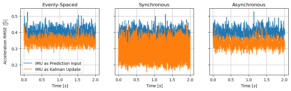
The following Monte Carlo runner simulates using four, 100 Hz IMUs with average measurement errors of \(0.5 \frac{m}{s^2}\) over two seconds with different types of time-synchronization to outline the scenarios where using IMU measurements as updates is detrimental and where it shows improvements. The following are descriptions of the different time synchronization modes.
1. Evenly-Spaced:
The measurements of the four IMUs are evenly spaced across a measurement period. In the case of four 100 Hz IMUs, this would be the equivalent of a single 400 Hz IMU. This is the best cause for using the measurements as Kalman prediction inputs, as there is no advantage from measurements being clustered and therefore correlated. The effect of filtering in this case is typically just to introduce a delay, which increases errors over the prediction input method.
2. Synchronous:
The measurements of the four IMUs are synchronized and all come in at identical times. This would be the case if there existing some external trigger, such as a GPS signal, to synchronize the IMU clocks. This is the worst case for using IMU measurements as inputs to the Kalman prediction, as you would be throwing away three of the four measurements at each step and just using whichever was last in the buffer. Conversely, this is the ideal scenario for a filter, as you could essentially take an average of the four measurements and have the equivalent of a lower-error sensor at the same original rate.
3. Asynchronous:
The initial measurement of each IMU is random within the range of the measurement period. This simulations a sensor being powered on and taking measurements as soon as possible with no form of clock synchronization, as is common if one were to just plug in multiple USB IMUs. This represents the most realistic scenario for non-synchronized multi-IMU systems and is therefore the most interesting for analysis. As will be shown, filtering takes advantage of the slight synchronization between the IMUs to develop more accurate predictions compared to using the last measurement alone.
def RMSE(input_array):
    np_array = np.array(input_array)
    return np.mean(np.sqrt(np.power(np_array, 2)), axis=0)

def run_simulation(n_sim, time_sync_type):
    err = 0.5
    rate = 100
    t_max = 2.0
    n_imu = 4

    pos_err_pred = []
    pos_err_filt = []
    vel_err_pred = []
    vel_err_filt = []
    acc_err_pred = []
    acc_err_filt = []

    for i in range(n_sim):
        all_t = np.array([])
        all_a = np.array([])
        for j in range(n_imu):
            imu_t = np.linspace(0, t_max, int(t_max * rate) + 1)

            if time_sync_type == 'evenly-spaced':
                # Measurements across IMUs are evenly spaced
                imu_t += j / n_imu / rate
            elif time_sync_type == 'synchronous':
                # Measurements across IMUs are perfectly synchronized
                imu_t += 0
            elif time_sync_type == 'asynchronous':
                # Each IMU's initial measurement time is randomly offset
                imu_t += np.random.uniform() / rate

            imu_a = acc_err(imu_t, err)

            all_t = np.concatenate([all_t, imu_t])
            all_a = np.concatenate([all_a, imu_a])

        all_t, all_a = (list(x) for x in \
            zip(*sorted(zip(all_t, all_a), key=lambda pair: pair[0])))

        pos_pred, vel_pred, acc_pred= predict(all_t, all_a)
        pos_filt, vel_filt, acc_filt, cov_filt = \
            filter(all_t, all_a, err, 1.0e3)

        pos_list_true = pos_true(all_t)
        vel_list_true = vel_true(all_t)
        acc_list_true = acc_true(all_t)

        pos_err_pred.append(np.array(pos_pred - pos_list_true))
        pos_err_filt.append(np.array(pos_filt - pos_list_true))
        vel_err_pred.append(np.array(vel_pred - vel_list_true))
        vel_err_filt.append(np.array(vel_filt - vel_list_true))
        acc_err_pred.append(np.array(acc_pred - acc_list_true))
        acc_err_filt.append(np.array(acc_filt - acc_list_true))

    pos_mean_pred = RMSE(pos_err_pred)
    pos_mean_filt = RMSE(pos_err_filt)
    vel_mean_pred = RMSE(vel_err_pred)
    vel_mean_filt = RMSE(vel_err_filt)
    acc_mean_pred = RMSE(acc_err_pred)
    acc_mean_filt = RMSE(acc_err_filt)

    return all_t, \
        pos_mean_pred, pos_mean_filt, \
        vel_mean_pred, vel_mean_filt, \
        acc_mean_pred, acc_mean_filt

# Run all simulations
t_0, p_pred_0, p_filt_0, v_pred_0, v_filt_0, a_pred_0, a_filt_0 = \
    run_simulation(100, 'evenly-spaced')

t_1, p_pred_1, p_filt_1, v_pred_1, v_filt_1, a_pred_1, a_filt_1 = \
    run_simulation(100, 'synchronous')

t_2, p_pred_2, p_filt_2, v_pred_2, v_filt_2, a_pred_2, a_filt_2 = \
    run_simulation(100, 'asynchronous')
Results
The following results show the root-mean-squared errors for position, velocity, and acceleration across all simulations using the two outlined methods in the de-synchronized, synchronized, and random start timing scenarios. As previously discussed, using IMU measurements purely as inputs to the Kalman prediction is beneficial in a multi-IMU system only when the measurements are evenly spaced and independent, which causes the system to behave as if there were only a single, higher rate, IMU. Using the IMU measurements as Kalman updates, however, shows large improvements if the IMU measurements are synchronized, or modest improvements in the more likely scenario where the measurements have random offsets in the start times.
In the most typical scenario of random start times, the resultant position, velocity, and acceleration errors are lowered by using the IMU measurements as Kalman updates instead of as inputs to the prediction step. This shows how, by making use of the slight correlation between closely spaced measurements, errors can be reduced by treating accelerations as a Kalman state and filtering the measurements on that state.
fig1, (axs1_0 ,axs1_1, axs1_2) = plt.subplots(1, 3, sharey=True)
axs1_0.set_title('Evenly-Spaced')
axs1_1.set_title('Synchronous')
axs1_2.set_title('Asynchronous')
axs1_0.plot(t_0, p_pred_0, label='IMU as Prediction Input')
axs1_0.plot(t_0, p_filt_0, label='IMU as Kalman Update')
axs1_1.plot(t_1, p_pred_1)
axs1_1.plot(t_1, p_filt_1)
axs1_2.plot(t_2, p_pred_2)
axs1_2.plot(t_2, p_filt_2)
axs1_0.set_ylabel(r'Position RMSE $$\left[ m \right]$$')
axs1_0.set_xlabel(r'Time $$\left[ s \right]$$')
axs1_1.set_xlabel(r'Time $$\left[ s \right]$$')
axs1_2.set_xlabel(r'Time $$\left[ s \right]$$')
axs1_0.legend()
axs1_0.grid(True)
axs1_1.grid(True)
axs1_2.grid(True)
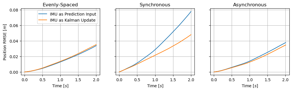
fig2, (axs2_0, axs2_1, axs2_2) = plt.subplots(1, 3, sharey=True)
axs2_0.set_title('Evenly-Spaced')
axs2_1.set_title('Synchronous')
axs2_2.set_title('Asynchronous')
axs2_0.plot(t_0, v_pred_0, label='IMU as Prediction Input')
axs2_0.plot(t_0, v_filt_0, label='IMU as Kalman Update')
axs2_1.plot(t_1, v_pred_1)
axs2_1.plot(t_1, v_filt_1)
axs2_2.plot(t_2, v_pred_2)
axs2_2.plot(t_2, v_filt_2)
axs2_0.set_ylabel(r'Velocity RMSE $$\left[ m \right]$$')
axs2_0.set_xlabel(r'Time $$\left[ s \right]$$')
axs2_1.set_xlabel(r'Time $$\left[ s \right]$$')
axs2_2.set_xlabel(r'Time $$\left[ s \right]$$')
axs2_0.legend()
axs2_0.grid(True)
axs2_1.grid(True)
axs2_2.grid(True)
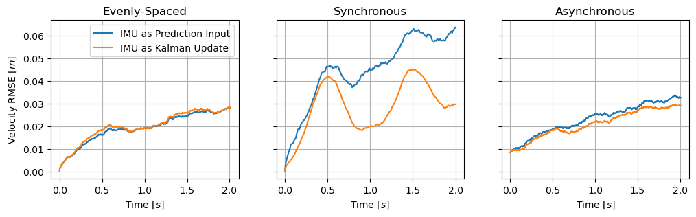
fig3, (axs3_0, axs3_1, axs3_2) = plt.subplots(1, 3, sharey=True)
axs3_0.set_title('Evenly-Spaced')
axs3_1.set_title('Synchronous')
axs3_2.set_title('Asynchronous')
axs3_0.plot(t_0, a_pred_0, label='IMU as Prediction Input')
axs3_0.plot(t_0, a_filt_0, label='IMU as Kalman Update')
axs3_1.plot(t_1, a_pred_1)
axs3_1.plot(t_1, a_filt_1)
axs3_2.plot(t_2, a_pred_2)
axs3_2.plot(t_2, a_filt_2)
axs3_0.set_ylabel(r'Acceleration RMSE $$\left[ \frac{m}{s^2} \right]$$')
axs3_0.set_xlabel(r'Time $$\left[ s \right]$$')
axs3_1.set_xlabel(r'Time $$\left[ s \right]$$')
axs3_2.set_xlabel(r'Time $$\left[ s \right]$$')
axs3_0.legend()
axs3_0.grid(True)
axs3_1.grid(True)
axs3_2.grid(True)
Conclusion
In conclusion, this work shows a simple example of how an asynchronous multi-IMU system can have lower position, velocity, and acceleration RMS errors by treating acceleration as a Kalman state, and utilizing incoming IMU measurements in the Kalman update step instead of as inputs to the Kalman prediction. This is by no means guaranteed, and is likely highly dependent on the types of motion the system is experiencing. Regardless, these results merit additional thought for multi-IMU systems.