This class was the second of my three undergraduate courses in dynamics and controls, where there was a distinct focus on controls, plant modeling, and transfer functions. This class introduced me to controls, and heightened my existing skills in dynamics. I also jumped head first into the first opportunity to apply my coding skills to more practical problems.

Labs 2 and 3

In this lab, a pendulum slider system was analyzed in order to better understand the modeling of dynamic systems using MatLab and Simulink software. Nonlinear and linear models were separately developed and simulated using both MatLab and Simulink and then compared to each other as well as an experimental measured response of the system. In the first part of the lab, the nonlinear and linear equations of motions were developed and simulated using MatLab and Simulink to predict the response of the system. It was shown that the simulations are identical in either programming environment and that under the small angle assumption, the linear system is a valid model. In the next part of the lab, the slider and pendulum position potentiometers were calibrated and data was collected after initiating motion in the system. The data was analyzed to find the coefficients of dry friction and viscous damping which were 0.0732 and 0.0968 respectively. Using these values to simulate the motion again on MatLab, the m Ns linear model, nonlinear model, and real response motions could be directly compared to determine the accuracy of the models. It was found that the coefficient of dry friction was verified, but the viscous damping coefficient had to be changed to 0.01 to produce a similar m Ns model to the experimental data. Therefore, it was shown that the methods used to calculate the coefficients are good for estimating, yet are not perfect. Additionally, the nonlinear model was shown to closely model the true to life experimental data that was collected in the lab, thus verifying the simulation techniques. Lab 2 & 3.

Labs 4 and 6

In this lab, a DC motor and inertial mass system was analyzed to better understand the modeling and implementation of open and closed loop controllers using MatLab and Simulink software. Open and closed loop controller simulations were created using calibration data and compared to experimental data. In the first section of the lab, the calibration data showed that both the potentiometer voltage and the motor response behaved linearly with the potentiometer Kx value as 17.589 [deg/V]. The second section of the lab showed that error is naturally induced in open loop controllers due to parameter uncertainty and that there are lower limitations on the motor speed. The data collected showed that both in simulations and implementations, the closed loop controller outperformed the open loop controller in regards to steady state error, confirming predictions. In the closed loop controller, the data showed that increasing the Kp value reduced the time constant of the system, but increased the steady state error. Finally, the comparisons between the modeled and experimental data confirmed the validity of the simulations used as models for the real world system. Lab 4 & 6.

Labs 5, 8, and 9

These three labs, Labs 5, 8, and 9, revolved around a real world problem of creating and implementing a system to control the level and flow rate of a coupled tank. This was done by first finding the mathematical model and numerical parameters of the coupled tank system. Then a simulation was ran so that a controller could be determined and refined through rapid iterations. From the information gathered in the first section of this lab, the PID controller for the system was initially determined to have the theoretical gain values of Kp = 6.7135, Ki = 1.0078, and Kd = 67.2116. After some refinement to make the model more linear, these values were adjusted to Kp = 35.7135, Ki = 0.0700, and Kd = 107.2116. Finally, this controller was implemented to manage both the level and the rise of water in the tank. In order for this controller to meet the specifications of a rise time being less than 15 seconds, a maximum overshoot being less than 20%, and a steady state error of 0, these gains were once again adjusted to the experimental values of Kp = 35.7135, Ki = 0.1000, and Kd = 107.2116. As a result of all of these adjustments, a controller was created that could adequately control the coupled tank system. Lab 5, 8 & 9.

Labs 10 and 11

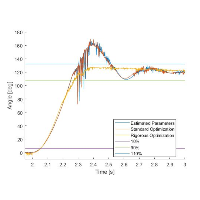
Labs 10 and 11 revolve around the design and implementation of a position controller for a DC motor. In Lab 10, a proportional-derivative (PD) controller was created to meet the desired specifications of a rise time of 10% of the time constant of the DC motor measured in Lab 4 in addition to a maximum percent overshoot of 10%. The original gain values used in the PD controller were 1.2059*10^4 and 33.1504 for Kp and Kd . This controller was then simulated in both MATLAB and Simulink in iterations until the specifications were met in both programs. The resulting gain values that were determined were Kr = 12000 and Kd = 58. The an even more rigorous DC motor model, these gain values were changed even more via iteration to Kp = 18000 and Kd = 1000. In Lab 11, this controller was then implemented into a DC motor in order to power it and turn it by a desired angle. While the system was able to reach the desired angle with a correct amount of overshoot, due to power limitations, the rise time could never be adjusted below the maximum allowed value of 0.0145. That being said, it was determined that this controller could be used to accurately change the motors position without much overshoot, with each of the gain values sets resulting in phase margins for small angles of 39.33 deg, 34.15 deg, and 80.30 deg and phase margins for large angles of 29.12 deg, 27.21 deg, and 64.93 deg respectively as the sets were presented here. Lab 10 & 11.